(MLOps) MLFlow 기초 - 실행 및 로깅

이 글은 에이콘 출판사의 ‘MLFlow를 활용한 MLOps’ 도서의 내용을 참고해 작성되었습니다.
MLOps란?
‘Machine Learning Operations’의 약자로, 데이터 적재, 전처리, 모델 훈련, 모델 저장, 테스트와 검증, 모델 배포, 모니터링 등 머신러닝의 생명주기에 포함된 모든 과정과 이를 효율적으로 관리하는 방법론을 통칭한다.
MLOps 엔지니어가 이 모든 과정을 담당한다면 리서처들은 데이터의 활용, 모델의 설계, 연구와 같은 과정에만 전념할 수 있게 된다. 특히 데이터 중심의 AI가 각광받음에 따라서 데이터의 품질 관리가 점점 중요해지고 있기에 연구자들이 고품질의 데이터를 활용할 수 있도록 돕는 MLOps 엔지니어의 역할이 더욱 커지는 상황이라고 생각한다. 물론 다양한 MLOps관련 도구에서 실험과 연관된 막강한 기능들을 지원하니, 연구자라도 스스로 MLOps에 대한 이해가 높다면 더욱 효율적인 실험 진행도 가능할 것이다!
개념 자체는 소프트웨어의 생명 주기를 책임지는 과정인 DevOps와 비슷하지만, 코드 중심이 아닌 데이터와 모델 중심의 관리라는 점에서 약간의 차이가 있다.
MLFlow란?
MLFlow는 대중적인 MLOps 오픈소스 라이브러리 중 하나이다. 강력한 로깅과 트래킹 기능, 도커와 콘다를 포함한 가상환경 파이프라인의 재사용성 확보, 모델 저장과 서버 배포 관리, 다양한 API와 UI기능 지원을 통한 확장성까지 이름처럼 머신러닝의 ‘흐름’에 필요한 다양한 기능을 활용할 수 있다. 깃헙 레포지터리 링크
MLFlow 설치
MLFlow 설치는 번거로운 과정 없이 pip를 통해 가능하다.
python3 -m pip install mlflow
붓꽃 데이터 로지스틱 회귀 예제
먼저, 필요한 데이터와 붓꽃 데이터를 불러온다.
import numpy as np
import pandas as pd
import matplotlib.pyplot as plt
import seaborn as sns
from sklearn.linear_model import LogisticRegression
from sklearn.model_selection import train_test_split
from sklearn.preprocessing import StandardScaler
from sklearn.metrics import confusion_matrix
from sklearn.datasets import load_iris

import mlflow
import mlflow.sklearn
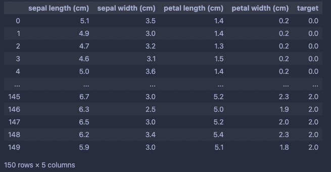
데이터를 판다스 데이터프레임으로 변환한다.
iris = load_iris()
iris_data = pd.DataFrame(data=np.c_[iris['data'], iris['target']], columns=iris['feature_names']+['target'])
iris_data
컬럼을 feature와 target으로 분할한다.
x_data = iris_data.iloc[:, :-1]
y_data = iris_data.iloc[:,[-1]]
클래스별로 변수를 따로 할당한다.
setosa = iris_data[iris_data.target == 0.0]
versicolor = iris_data[iris_data.target == 1.0]
virginica = iris_data[iris_data.target == 2.0]

print("Setosa : {}".format(setosa.shape))
print("Versicolor : {}".format(versicolor.shape))
print("Virginica : {}".format(virginica.shape))
>>>
Setosa : (50, 5)
Versicolor : (50, 5)
Virginica : (50, 5)
훈련셋과 테스트셋으로 분할한다.
setosa_train, setosa_test = train_test_split(setosa, test_size=0.2)
versicolor_train, versicolor_test = train_test_split(versicolor, test_size=0.2)
virginica_train, virginica_test = train_test_split(virginica, test_size=0.2)
나눴던 변수를 다시 concat한다.
x_train = pd.concat((setosa_train, versicolor_train, virginica_train))
x_test = pd.concat((setosa_test, versicolor_test, virginica_test))

y_train = np.array(x_train['target'])
y_test = np.array(x_test['target'])

x_train.drop('target', axis=1, inplace=True)
x_test.drop('target', axis=1, inplace=True)
>>>
Training sets:
	x_train: (120, 4)
	y_train: (120,)

Testing sets:
	x_test: (30, 4)
	y_test: (30,)
피처 스케일링
scaler = StandardScaler()
scaler.fit(pd.concat((setosa, versicolor, virginica)).drop('target', axis=1))
x_train = scaler.transform(x_train)
x_test = scaler.transform(x_test)
훈련 함수 작성
def train(sklearn_model, x_train, y_train):
    sklearn_model = sklearn_model.fit(x_train, y_train)
    train_acc = sklearn_model.score(x_train, y_train)
    mlflow.log_metric("train_acc", train_acc)
    print("Train Accuracy: {:.3%}".format(train_acc))
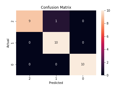
평가 함수 작성
def evaluate(sklearn_model, x_test, y_test):
    eval_acc = sklearn_model.score(x_test, y_test)
    preds = sklearn_model.predict(x_test)

    mlflow.log_metric("eval_acc", eval_acc)
    print("Eval Accuracy: {:.3%}".format(eval_acc))

    conf_matrix = confusion_matrix(y_test, preds)
    ax = sns.heatmap(conf_matrix, annot=True, fmt='g')
    ax.invert_xaxis()
    ax.invert_yaxis()
    plt.ylabel('Actual')
    plt.xlabel('Predicted')
    plt.title("Confusion Matrix")
    plt.savefig("sklearn_conf_matrix.png")
    mlflow.log_artifact("sklearn_conf_matrix.png")
모델과 실험(파이프라인)을 설정한다.
처음에 mlflow.set_experiment("실험이름")을 통해 로깅될 실험의 이름을 설정한다.
with 블록 안에 파이프라인 train, evaluate, logging 등의 과정이 적재되어있고, start_run() 메소드를 통해 실행된다. with 구문 덕분에 각 실행의 독립성이 보장된다. 쉽게 말해 여러번 실험을 할 경우 하나의 실험이 예상치 못하게 종료되든, 올바르게 종료되든 다음 실험에는 전혀 영향을 주지 않는다.
sklearn_model = LogisticRegression(max_iter=50, solver='newton-cg')
mlflow.set_experiment("iris_experiment")
with mlflow.start_run():
    train(sklearn_model, x_train, y_train)
    evaluate(sklearn_model, x_test, y_test)
    mlflow.sklearn.log_model(sklearn_model, "log_reg_model")
    print("Model run: ", mlflow.active_run().info.run_uuid)
mlflow.end_run()
MLFlow는 이처럼 pythonic한 파이프라인을 작성하기 좋다.
실행결과는 다음과 같다
>>>
Train Accuracy: 95.000%
Eval Accuracy: 96.667%
Model run:  e45b49292ea64807844ccd436d379672
loaded_model = mlflow.sklearn.load_model("runs:/a67105e9dd424de390b33509cc1a7e10/log_reg_model")
print(loaded_model.score(x_test, y_test))
>>>
0.9666666666666667
MLFlow ui 실행
터미널 접속 후 코드가 저장된 디렉토리에서
mlflow ui -p 9999 # 포트 번호 지정
만약 command not found 에러를 마주한다면 conda(miniforge) 가상환경이 활성화가 된 상태인지 먼저 확인해보자.
정상적으로 진행된다면 다음과 같이 localhost의 9999번 포트에서 실행된다.
[2022-04-12 22:07:09 +0900] [9424] [INFO] Starting gunicorn 20.1.0
[2022-04-12 22:07:09 +0900] [9424] [INFO] Listening at: http://127.0.0.1:9999 (9424)
[2022-04-12 22:07:09 +0900] [9424] [INFO] Using worker: sync
[2022-04-12 22:07:09 +0900] [9425] [INFO] Booting worker with pid: 9425
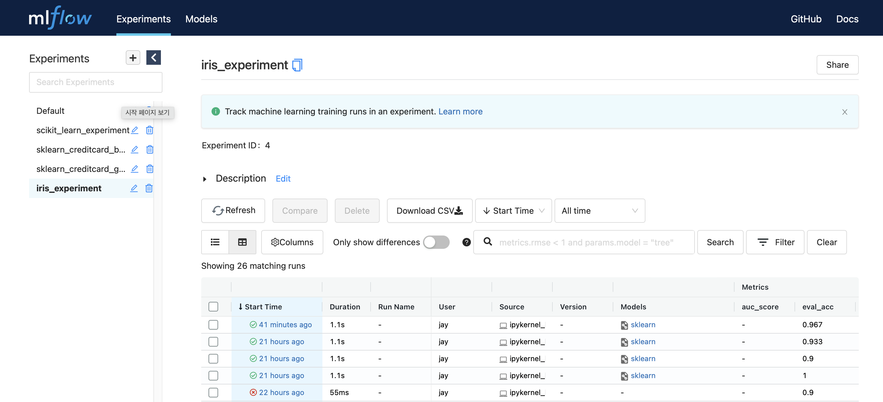
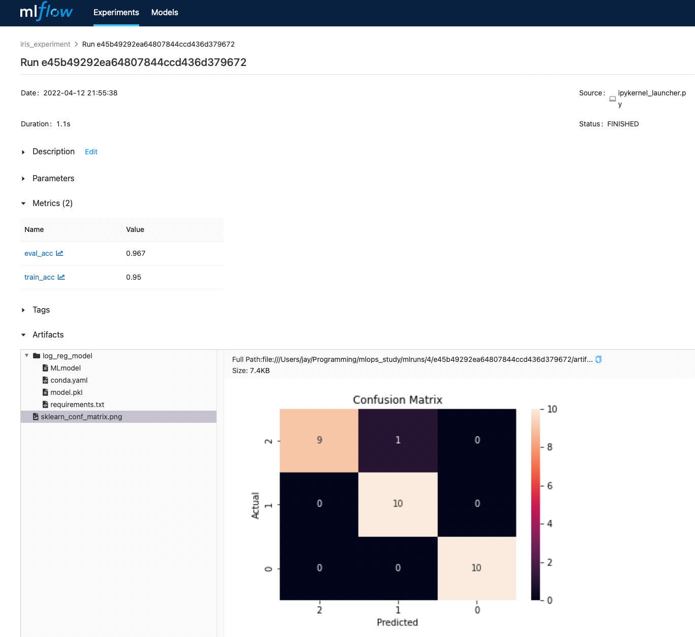
왼쪽에 실험명인 iris_experiment를 클릭하면 그동안의 실험이 전부 기록되어 있다.
가장 최근의 실행을 클릭해 들어가보면 기록된 설명, 파라미터, 평가항목, 태그, 저장된 모델 정보와 이미지 등을 볼 수 있다.
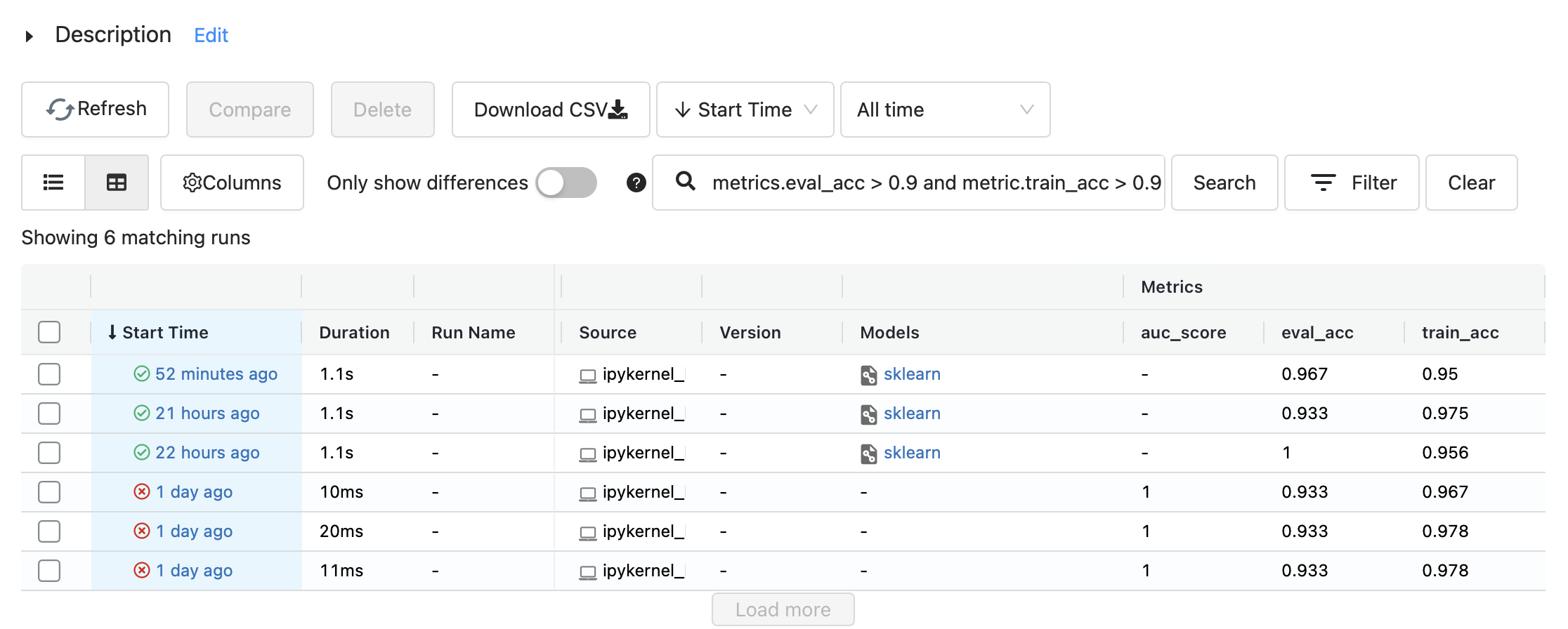
다음과 같이 필터링 조건을 걸어 원하는 실행만 모아 볼 수 있고
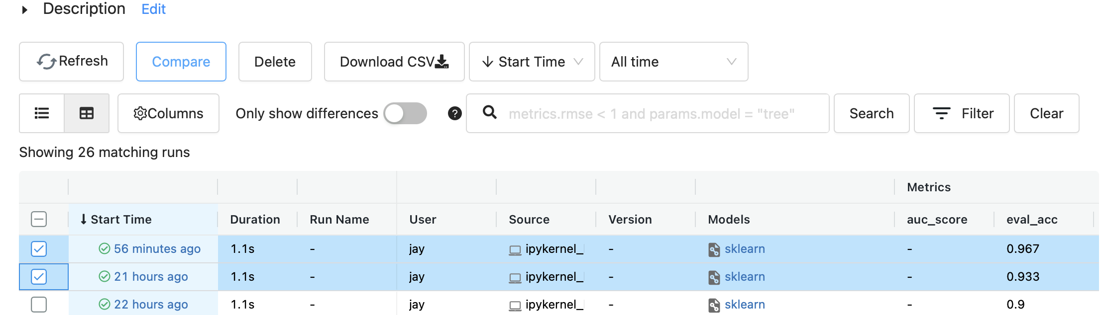
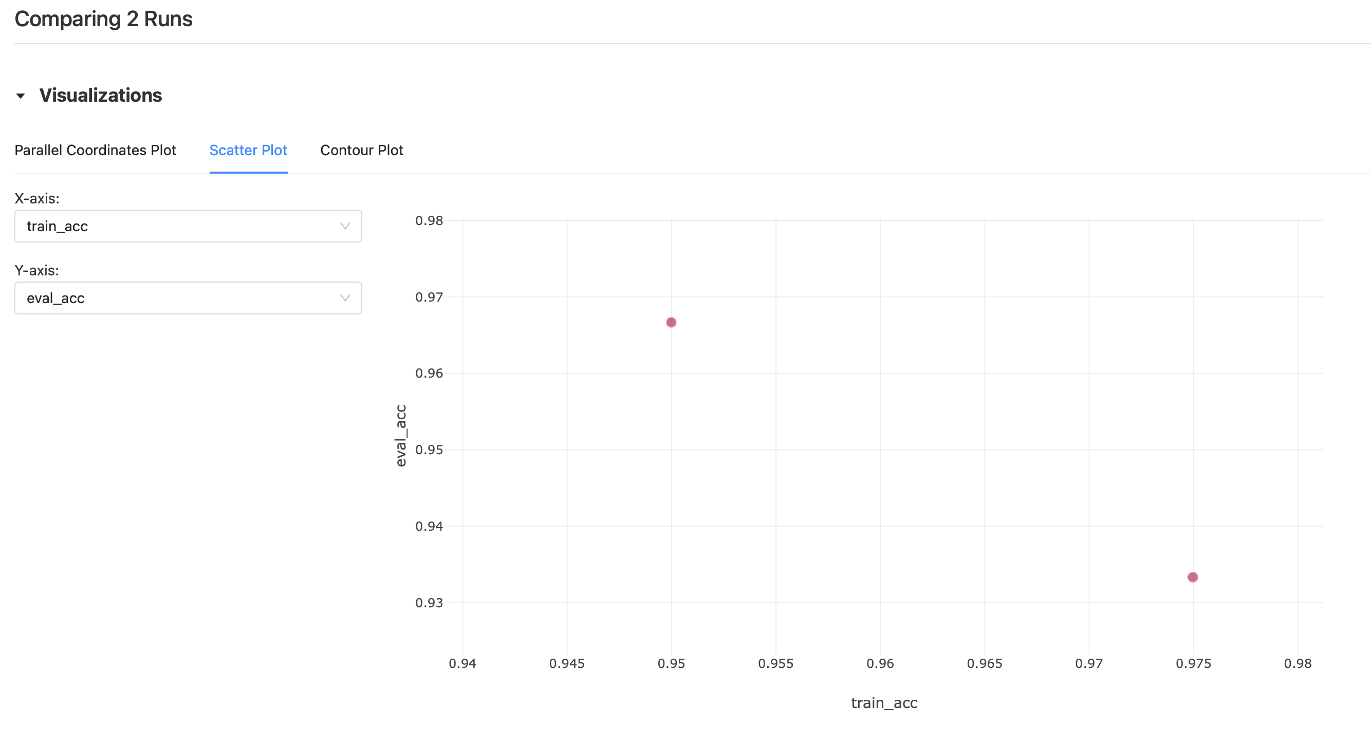
여러개의 실행을 동시 선택 후 Compare를 눌러 실행간의 시각화된 비교 결과를 볼 수 도 있다.
좌측 실험 탭에서 각 실험들은 휴지통 버튼으로 삭제할 수 있지만, 삭제된 실험들은 모두 .trash에 남아있다. 따라서 완전히 삭제하기 위해선 터미널에서 따로 휴지통을 비워줘야 한다.
rm -rf mlruns/.trash/*
터미널에서 포그라운드 상태로 ‘ctrl + c’를 눌러 MLFlow를 종료할 수 있다. 맥에서도 ‘command’가 아닌 ‘ctrl’을 그대로 사용하면 된다.
또는 pkill -f gunicorn 으로도 종료할 수 있다.
출처
'mlops' 카테고리의 다른 글
더보기| (MLOps) MLFlow 기초 - 모델 배포 및 쿼리 | 2022. 05. 09 |
|---|---|
| (MLOps) MLFlow 기초 - 실행 및 로깅 | 2022. 04. 12 |